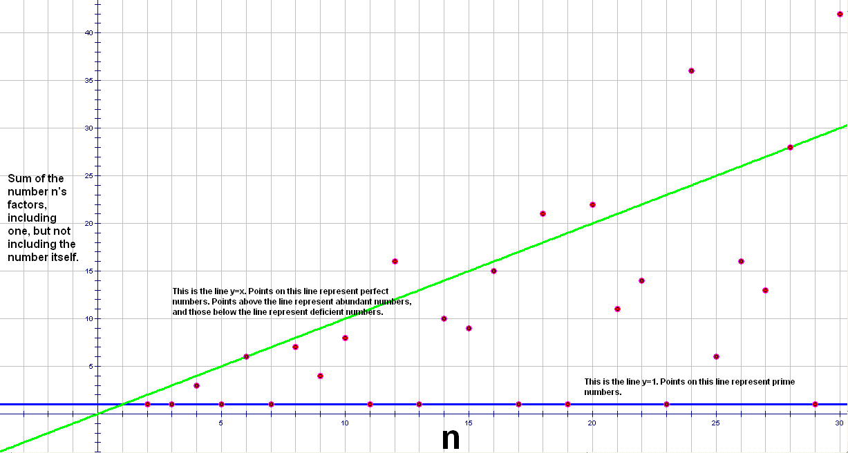
In this graph, each number on the x-axis (from 2 to 30) is plotted against the sum of all its factors (including one, but excluding the number itself) on the y-axis. Numbers on the blue line y = 1 have no factors other than one and themselves, and are therefore prime numbers. Numbers on the green line y = x are equal to the sum of their factors (including one, but excluding themselves), and are therefore perfect numbers. Perfect numbers are much rarer than prime numbers in the entire set of natural numbers, as well as in this small sample.

If a number’s factor-sum, examined in this manner, is smaller than the number itself, such a number is called a “deficient number.” This applies to all numbers with points below the green line. Numbers which have points on the blue line are deficient numbers, as well as being prime numbers – and this is true for all prime numbers, no matter how large. The numbers represented by points between the green and blue lines are, therefore, both deficient and composite, and can also be called “non-prime deficient numbers.”

A few numbers on this graph, called “abundant numbers,” are represented by points above the green line, because their factor-sum is greater than the number itself. There are only five abundant numbers in this sample: 12, 18, 20, 24, and 30. As an example of how a number is determined to be abundant, consider the factors of 30: 1+2+3+5+6+10+15 = 42, which is, of course, greater than 30.

Of the 29 numbers examined in this sample, here is how they break down by category:

• Abundant numbers: 5 (~17.2% of the total)
• Perfect numbers: 2 (~6.9% of the total)
• Non-prime deficient numbers: 12 (~41.4% of the total)
• Prime numbers: 10 (~34.4% of the total)

These percentages only add up to 99.9%, due simply to rounding. Also, the total number of deficient numbers in this sample (both prime and composite) is 22, which is ~75.9% of the total sample of 29 numbers.

So what happens if this survey is extended far beyond the number 30, to analyze much larger (and therefore more meaningful) samples? Well, for one thing, the information on the graph above would quickly become too small to read, but that is only of trivial importance. More significantly, what would happen to the various percentages, for each category, given above? First, both prime and perfect numbers become more difficult to find, as larger and larger numbers are examined – so the percentages for these categories would shrink dramatically, especially the one for perfect numbers. With smaller percentages of prime and perfect numbers in much larger samples, the sum of the percentages for the other two categories (abundant and non-prime deficient numbers) would, of necessity, grow larger. That has to be true for this sum – but that says nothing about what would happen to its two individual components. My guess is that abundant numbers would become more common in larger samples . . . but since I have not yet examined the data, I’m only calling this a guess, not even a conjecture. As for what would happen to the percentage of non-prime deficient numbers when larger samples are analyzed, I don’t even (yet) have a guess.