A Truncated Octahedron, with Pyramids Excavated from the Square Faces

Posted on 7 July 2014 by RobertLovesPi

I used Stella 4d, available at http://www.software3d.com/Stella.php, to make this.

Ring of Eight Great Rhombcuboctahedra

Posted on 7 July 2014 by RobertLovesPi

I used Stella 4d, available at http://www.software3d.com/Stella.php, to make this.

A Graphical Survey of Prime, Perfect, Deficient, and Abundant Numbers From Two to Thirty

Posted on 5 July 2014 by RobertLovesPi

In this graph, each number on the x-axis (from 2 to 30) is plotted against the sum of all its factors (including one, but excluding the number itself) on the y-axis. Numbers on the blue line y = 1 have no factors other than one and themselves, and are therefore prime numbers. Numbers on the green line y = x are equal to the sum of their factors (including one, but excluding themselves), and are therefore perfect numbers. Perfect numbers are much rarer than prime numbers in the entire set of natural numbers, as well as in this small sample.

If a number’s factor-sum, examined in this manner, is smaller than the number itself, such a number is called a “deficient number.” This applies to all numbers with points below the green line. Numbers which have points on the blue line are deficient numbers, as well as being prime numbers – and this is true for all prime numbers, no matter how large. The numbers represented by points between the green and blue lines are, therefore, both deficient and composite, and can also be called “non-prime deficient numbers.”

A few numbers on this graph, called “abundant numbers,” are represented by points above the green line, because their factor-sum is greater than the number itself. There are only five abundant numbers in this sample: 12, 18, 20, 24, and 30. As an example of how a number is determined to be abundant, consider the factors of 30: 1+2+3+5+6+10+15 = 42, which is, of course, greater than 30.

Of the 29 numbers examined in this sample, here is how they break down by category:

• Abundant numbers: 5 (~17.2% of the total)
• Perfect numbers: 2 (~6.9% of the total)
• Non-prime deficient numbers: 12 (~41.4% of the total)
• Prime numbers: 10 (~34.4% of the total)

These percentages only add up to 99.9%, due simply to rounding. Also, the total number of deficient numbers in this sample (both prime and composite) is 22, which is ~75.9% of the total sample of 29 numbers.

So what happens if this survey is extended far beyond the number 30, to analyze much larger (and therefore more meaningful) samples? Well, for one thing, the information on the graph above would quickly become too small to read, but that is only of trivial importance. More significantly, what would happen to the various percentages, for each category, given above? First, both prime and perfect numbers become more difficult to find, as larger and larger numbers are examined – so the percentages for these categories would shrink dramatically, especially the one for perfect numbers. With smaller percentages of prime and perfect numbers in much larger samples, the sum of the percentages for the other two categories (abundant and non-prime deficient numbers) would, of necessity, grow larger. That has to be true for this sum – but that says nothing about what would happen to its two individual components. My guess is that abundant numbers would become more common in larger samples . . . but since I have not yet examined the data, I’m only calling this a guess, not even a conjecture. As for what would happen to the percentage of non-prime deficient numbers when larger samples are analyzed, I don’t even (yet) have a guess.

Black and White Tessellation Using Semicircles

Image

All of the curves used in this tessellation are semicircles. The tessellation itself is a modification of the regular tessellation of the plane using equilateral triangles.

Polyhedron with 362 Faces

Image

Polyhedron with 362 Faces

I’d like to find a polyhedron with the same number of faces as there are days of the year. This is the closest I’ve come, so far.

The software I used, Stella 4d, may be purchased at http://www.software3d.com/Stella.php. There is also a free trial download available.

A Simulation of Crystalline Growth Using Polyhedral Augmentation

Posted on 29 June 2014 by RobertLovesPi

Crystals and crystalline growth have been studied for centuries because of, at least in part, their symmetry. Crystals are cut in such a way as to increase this symmetry even more, because most people find symmetry attractive. However, where does the original symmetry in a crystal come from? Without it, jewelers who cut gemstones would not exist, for the symmetry of crystalline minerals themselves is what gives such professionals the raw materials with which to work.

To understand anything about how crystals grow, one must look at a bit of chemistry. The growth of crystals:

Involves very small pieces: atoms, molecules, ions, and/or polyatomic ions
Involves a small set of simple rules for how these small pieces attach to each other

Why small pieces? That’s easy: we live in a universe where atoms are tiny, compared to anything we can see. Why is the number of rules for combining parts small, though? Well, in some materials, there are, instead, large numbers of ways that atoms, etc., arrange themselves — and when that happens, the result, on the scale we can see, is simply a mess. Keep the number of ways parts can combine extremely limited, though, and it is more likely that the result will possess the symmetry which is the source of the aesthetic appeal of crystals.

This can be modeled, mathematically, by using polyhedral clusters. For example, I can take a tetrahedron, and them augment each of its four faces with a rhombicosidodecahedron. The result is this tetrahedral cluster:

Next, having chosen my building blocks, I need a set of rules for combining them. I choose, for this example, these three:

Only attach one tetrahedral cluster of rhombicosidodechedra to another at triangular faces — and only use those four triangles, one on each rhombicosidodecahedron, which are at the greatest distance from the cluster’s center.
Don’t allow one tetrahedral cluster to overlap another one.
When you add a tetrahedral cluster in one location, also add others which are in identical locations in the overall, growing cluster.

Using these rules, the first augmentation produces this:

That, in turn, leads to this:

Next, after another round of augmentation:

One more:

In nature, of course, far more steps than this are needed to produce a crystal large enough to be visible. Different crystals, of course, have different shapes and symmetries. How can this simulation-method be altered to model different types of crystalline growth? Simple: use different polyhedra, and/or change the rules you select as augmentation guidelines, and you’ll get a different result.

[Note: all of these images were created using Stella 4d: Polyhedron Navigator. This program is available at http://www.software3d.com/Stella.php.]

Sprawling Clusters of Truncated Tetrahedra

Posted on 29 June 2014 by RobertLovesPi

Truncated tetrahedra make interesting building blocks. In the images below, the truncated tetrahedron “atoms” are grouped into four-part “molecules,” each with a triangular face pointed toward the molecular center, which is found in a small tetrahedral hole between the four truncated tetrahedra. These four-part “molecules” are then attached to other, always with three coplanar triangular faces from one “molecule” meeting three from the other. If you start from a central “molecule,” and let such a cluster grow for a small number of iterations, you get this:

What does the cluster above look like if even more truncated tetrahedra are added, but without allowing overlap to occur? Like this:

Like the truncated tetrahedron itself, these sprawling clusters have tetrahedral symmetry. To keep such symmetry while building these clusters, of course, one must be careful about the exact placement of the pieces — and doing this becomes more difficult as the cluster grows ever larger. I was able to take this one more step:

All of these images were created using Stella 4d: Polyhedron Navigator. This program is available at http://www.software3d.com/Stella.php.

Multiple Octahedra, in a Rotating Cluster with Tetrahedral Symmetry

Image

Multiple Octahedra, in a Rotating Cluster with Tetrahedral Symmetry

I created this cluster using Stella 4d: Polyhedron Navigator. This program is available at http://www.software3d.com/Stella.php.

A Comparison of the Areas of Some of the Triangles Formed By Connecting Three Noncollinear Triangle Centers

Posted on 28 June 2014 by RobertLovesPi

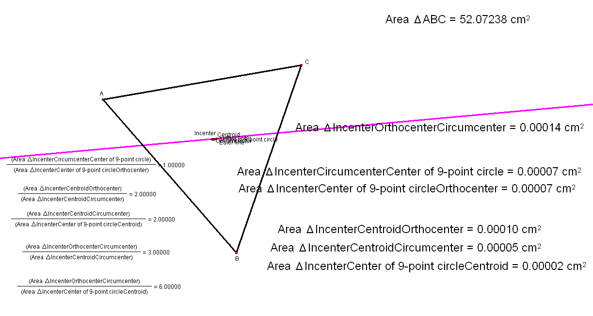
The five most well-known triangle centers are the centroid (where a triangle’s medians meet), the orthocenter (where the lines containing the altitudes meet), the incenter (where a triangle’s three interior angle bisectors meet), the circumcenter (where the perpendicular bisectors of a triangle’s three sides meet), as well as the center of a triangle’s 9-point circle (see https://en.wikipedia.org/wiki/Nine-point_circle for more information on this circle, and how it is defined). In the diagram below, the constructions for all five of these triangle centers have been performed, for obtuse, scalene triangle ABC.

The thick pink line is called the Euler line, and four of the five triangle centers mentioned above — all of them except the incenter — are always located on this line, no matter a triangle’s shape or size. The incenter, however, is only found on the Euler line for isosceles or equilateral triangles, so, for such triangles, all five of these triangle centers are collinear — and, as a consequence, no triangles can be made by connecting any set of three of them. If the triangle is scalene, however, the incenter will leave the Euler line, and these triangles may then be defined (with construction-clutter removed, but for the same triangle ABC as shown in the first diagram):

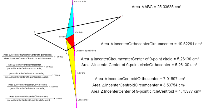
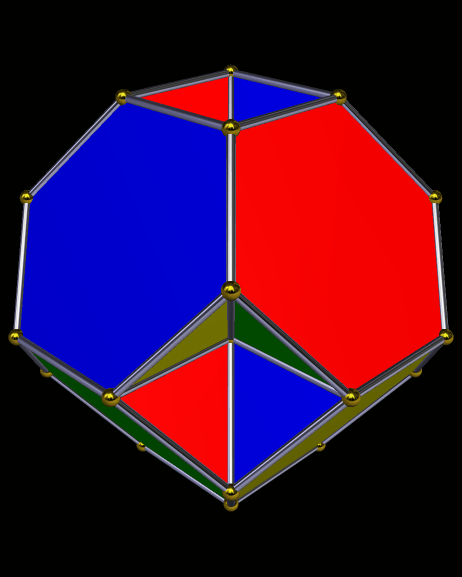
If A, B, and/or C are moved around, the area of triangle ABC changes, as do, of course, the areas of the colored triangles above, of which there are six: yellow, red, blue, yellow and red together, blue and red together, and all three taken as one triangle. For the original configuration of triangle ABC, you can see those triangle areas on the right side of the image above. On the left side, various ratios are given:

The triangle which joins the incenter, 9-point circle center, and circumcenter has the same area as the triangle joining the incenter, 9-point circle center, and the orthocenter.
The triangle joining the incenter, centroid, and orthocenter has twice the area of the triangle joining the incenter, centroid, and circumcenter — and this latter triangle, itself, has twice the area of the triangle joining the incenter, centroid, and 9-point circle center.
The area of the triangle connecting the incenter, orthocenter, and circumcenter has an area three times as large as the triangle connecting the incenter, centroid, and circumcenter.
As a consequence of the last two bulleted statements, the area of the triangle connecting the incenter, orthocenter, and circumcenter is six times the area of the triangle connecting the incenter, centroid, and 9-point circle center.

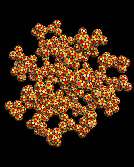
In both diagrams above, the original triangle ABC is scalene and obtuse. If A, B, and/or C are moved around, but the triangle remains scalene (so that the five triangle centers in question remain noncollinear), all six of the colored triangles described above still exist — and the area ratios given in the bulleted statements above remain constant, also. I do not yet have proofs for the constancy of these area ratios, but am confident that it is possible to write them.

If A, B, and C are positioned in such a way that triangle ABC is almost equilateral, the five triangle centers discussed here get very close together — because for a triangle which actually is regular, all five are located in exactly the same spot. Here’s what the almost-regular case looks like:

As you can see, the area ratios described above (left side of diagram) remain the same, even as the actual colored-triangle areas (right side) all approach zero. If I complete a proof for the constancy of any or all of these area ratios, I’ll post such proofs in subsequent posts on this blog — or readers are welcome to write their own proofs, and are invited to leave them as comments on this post.

Four Octahedra, Rotating in Tetrahedral Formation

Image

Four Octahedra, Rotating in Tetrahedral Formation

I created this cluster by augmenting each face of a tetrahedron with an octahedron, using Stella 4d: Polyhedron Navigator. This program is available at http://www.software3d.com/Stella.php.