Circumsinusoidal Regions, Part Two

Posted on 19 July 2014 by RobertLovesPi

[Note: If you haven’t yet read part one, it is recommended to read it first, before reading this part. Part one is the most recent post here, before this one.]

In part one, a special circumsinusoidal region was described, bounded by parts of semicircles, and a sine or cosine wave. As previously described, this requires that the wave’s amplitude be exactly one-fourth the wavelength. Of course, most sinusoidal waves do not have amplitudes and wavelengths that fall nicely into a 1:4 ratio. What happens, then, with the majority of waves — the ones with with other amplitude:wavelength ratios? Can they still be used for forming circumsinusoidal regions? The answer is yes — but the cost required is that semicircles may no longer by used in their construction.

A semicircle can be thought of as a 180 degree arc, if the diameter, often considered part of its perimeter, is ignored. When the sine or cosine wave’s amplitude:wavelength ratio is not equal to 1:4, the only necessary adjustments for the circular arcs needed to define particular circumsinusoidal regions are identical changes in the angular size of each arc used, plus translations of the centers of the circles which contain each of these circular arcs. These translations move those circle-centers away from the line representing the wave’s rest position, in a direction perpendicular to that line. There are two cases to consider: shorter-amplitude waves (those with an amplitude:wavelength ratio smaller than 1:4), and taller-amplitude waves (where the same ratio is greater than 1:4). The first picture below shows the shorter-amplitude case.

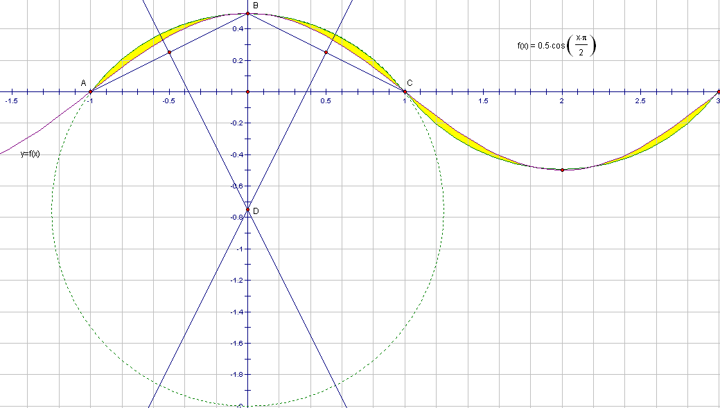
For every half-wavelength which starts at the rest position, an arc through three points is needed for the outer bound of the circumsinusoidal regions, which are shown in yellow. Those three points are two consecutive points (such as A and C above) where the sinusoidal wave crosses the rest position, plus the point at the top of the wave crest (such as B), or the point at the bottom of the trough, exactly half-way along the sinusoidal curve, in-between the two consecutive rest-position points under examination. In this example using points A, B, and C, above, the circle containing those points was constructed by drawing segments AB and BC, and then constructing the perpendicular bisectors of those two segments. Thone perpendicular disectors intersect at some point D, which is the center of a circle containing A, B, and C. The part of this circle which is not used for the arc through A, B, and C is shown as a dashed arc, while the arc used is shown as a solid curve. For other half-waves, to the left or right of this circle and arc, the construction would proceed in the same fashion, but is not shown, for the sake of clarity.

The taller-wavelength case also can be constructed, using the same procedure, as shown below.

These regions, of course, have area. To determine the exact area of any circumsinusoidal region requires integral calculus, and this area is equal to the difference in the areas under two different types of curve. Without calculus, the best that can be found for these areas are mere approximations, not exact answers. I am leaving this find-the-area problem for mathematicians who have a better understanding of calculus than I possess.

Circumsinusoidal Regions, Part One

Posted on 19 July 2014 by RobertLovesPi

The inner boundary of the yellow regions above is a sine curve (technically, a cosine curve, but that’s the same thing, just with a phase shift). The outer boundaries are semicircles. In order for this to work, to form these yellow regions, the semicircle centers (centers of the circles they are each half of) must be directly below peaks, and above troughs, of the sine (or cosine) curve, and vertically positioned at what would be called the rest position in physics. (I’m resorting to use of some physics terminology here, simply because I don’t know the corresponding mathematical terms).

In addition, each semicircle involved must have a radius equal to one-fourth the wavelength of the sine or cosine wave. The two sets of curves cross each other at the rest position, and are tangent to each other at each peak and trough, producing four of these yellow regions per wavelength.

In this case, semicircles could used because I adjusted the wavelength, making it exactly four times the amplitude of the wave. My goal was to compare the two curves, simply to see how well one simulates the other (answer: not very well at all). Then, however, I became more interested in the discrepancy between the two, represented by the yellow regions which are outside the true wave, and inside the semicircles which contain that wave. Until and unless I find that such regions already have a different name, I am naming these two-dimensional curved shapes “circumsinusoidal regions.” There are four of them per wavelength of the wave, and two per semicircle. Each circumsinusoidal region has two vertices, but the two paths connecting them are distinct curves. No part of either path contains any length which is a straight segment.

It would be possible to generate interesting solids by rotating circumsinusoidal regions around vertical or horizontal lines, such as the x- or y-axes, or around diagonal lines. Many such solids would be variations of a torus, including the central hole of a torus, but with circumsinusoidal cross-sections replacing a torus’s circular cross-sections. Unfortunately, I do not have the software I would need to generate pictures of such solid figures.

If the wavelength used for a given sinusoidal wave is not exactly four times the wave’s amplitude, semicircles won’t work to enclose the wave with the same points of tangency, but it is still possible to generate circumsinusoidal regions — using something, in their place, other than semicircles. This will be described in part two, which will be the next post on this blog.

A Comparison of the Areas of Some of the Triangles Formed By Connecting Three Noncollinear Triangle Centers

Posted on 28 June 2014 by RobertLovesPi

The five most well-known triangle centers are the centroid (where a triangle’s medians meet), the orthocenter (where the lines containing the altitudes meet), the incenter (where a triangle’s three interior angle bisectors meet), the circumcenter (where the perpendicular bisectors of a triangle’s three sides meet), as well as the center of a triangle’s 9-point circle (see https://en.wikipedia.org/wiki/Nine-point_circle for more information on this circle, and how it is defined). In the diagram below, the constructions for all five of these triangle centers have been performed, for obtuse, scalene triangle ABC.

The thick pink line is called the Euler line, and four of the five triangle centers mentioned above — all of them except the incenter — are always located on this line, no matter a triangle’s shape or size. The incenter, however, is only found on the Euler line for isosceles or equilateral triangles, so, for such triangles, all five of these triangle centers are collinear — and, as a consequence, no triangles can be made by connecting any set of three of them. If the triangle is scalene, however, the incenter will leave the Euler line, and these triangles may then be defined (with construction-clutter removed, but for the same triangle ABC as shown in the first diagram):

If A, B, and/or C are moved around, the area of triangle ABC changes, as do, of course, the areas of the colored triangles above, of which there are six: yellow, red, blue, yellow and red together, blue and red together, and all three taken as one triangle. For the original configuration of triangle ABC, you can see those triangle areas on the right side of the image above. On the left side, various ratios are given:

The triangle which joins the incenter, 9-point circle center, and circumcenter has the same area as the triangle joining the incenter, 9-point circle center, and the orthocenter.
The triangle joining the incenter, centroid, and orthocenter has twice the area of the triangle joining the incenter, centroid, and circumcenter — and this latter triangle, itself, has twice the area of the triangle joining the incenter, centroid, and 9-point circle center.
The area of the triangle connecting the incenter, orthocenter, and circumcenter has an area three times as large as the triangle connecting the incenter, centroid, and circumcenter.
As a consequence of the last two bulleted statements, the area of the triangle connecting the incenter, orthocenter, and circumcenter is six times the area of the triangle connecting the incenter, centroid, and 9-point circle center.

In both diagrams above, the original triangle ABC is scalene and obtuse. If A, B, and/or C are moved around, but the triangle remains scalene (so that the five triangle centers in question remain noncollinear), all six of the colored triangles described above still exist — and the area ratios given in the bulleted statements above remain constant, also. I do not yet have proofs for the constancy of these area ratios, but am confident that it is possible to write them.

If A, B, and C are positioned in such a way that triangle ABC is almost equilateral, the five triangle centers discussed here get very close together — because for a triangle which actually is regular, all five are located in exactly the same spot. Here’s what the almost-regular case looks like:

As you can see, the area ratios described above (left side of diagram) remain the same, even as the actual colored-triangle areas (right side) all approach zero. If I complete a proof for the constancy of any or all of these area ratios, I’ll post such proofs in subsequent posts on this blog — or readers are welcome to write their own proofs, and are invited to leave them as comments on this post.

A Triangle’s Tridpoint-Hexagon

Image

A Triangle's Tridpoint-Hexagon

Any triangle may be named triangle ABC. Each of its sides will contain exactly two points — called “tridpoints” — which divide that side into three segments of equal length. In triangle ABC above, the tridpoints are named in such a way that two of them, E and F, are encountered, in that order, if one moves from A to B. On the way from B to C, two more tridpoints are encountered: first F, and then G. Finally, going from C back to A, the last two tridpoints are found: first H, and then J. If a polygon is formed using those six tridpoints in alphabetical order (matching the order of their placement), that polygon is a convex hexagon, DEFGHJ. Another name for it is hexagon DJHGFE, which I mention only because Geometer’s Sketchpad called it that, in the picture above, when I asked it for the area of this hexagon, shown in green. The original triangle, ABC, includes both the yellow and green regions, and I asked Sketchpad for the area of this triangle, also, as well as the hexagon-to-triangle area ratio, which is shown above as the familiar “decimalized” version of the fraction 2/3.

A nice feature of Sketchpad is that you can do things like this — and then move points around, to see what effect that has on measured and calculated values. When I move points A, B, and/or C, the triangle and hexagon areas, of course, change. Their area ratio, however, remains at a decimal which is a rounded-off version of 2/3. It doesn’t change at all, no matter where A, B, and C are placed. Any triangle’s tridpoint-hexagon has an area exactly 2/3 that of the original triangle.

This is not yet a theorem — because what is written above is an explanation, not a proof. I’ve started working on a proof for this conjecture in my head, and will post it on this blog when/if I successfully complete it.

[Later edit — one of my readers provided a proof, so now it’s a theorem. For his proof, see the first comment on this post.]

Triangle Investigations

Posted on 27 June 2014 by RobertLovesPi

I just spent a couple of hours playing with triangles, their centers, and related things, using Geometer’s Sketchpad. Much of what I found was already known, but some of the things I found may not be. It will take more research to sort out which is which.

This is where I started. My original triangle, ABC, has heavy black sides and a yellow interior. The sides of ΔABC are extended as black dashed lines. I constructed ΔABC’s three angle bisectors to find its incenter, then constructed perpendicular lines to each side of the triangle from the incenter to find the three “touchpoints,” called A’, B’, and C’, allowing me to construct the incircle of my starting triangle. I also wanted the three excircles, and they are centered at A”, B”, and C” — the three excenters of triangle ABC. These points are found by bisecting all exterior angles of the original triangle, and then looking for the three point of concurrency among themselves, and the three interior angle bisectors previously used to locate the incenter. The heavy green, large triangle is the triangle which connects the three excenters, and probably has an established name, but I couldn’t find it — so I’ll just be calling it the “green triangle.” It is not to be confused with the small triangle in the diagram’s center, which has red sides and a green interior. This small triangle is simply formed by connecting the touchpoints A’, B’, and C’, and has several names already: the Gergonne triangle, the contact triangle, and the intouch triangle of ΔABC.

I set this up in such a way that I could move points A, B, and C around, and watch what happened to angle measures, segment lengths, areas, and area ratios. The picture above shows what happens near regularity, with all three interior angles very close to 60°. This is how I learned that certain area ratios are at a minimum when the triangle is equilateral — as you’ll see, they are all larger in subsequent pictures. At regularity, the green triangle has an area exactly four times that of the original triangle, which, in turn, has an area four times larger than the Gergonne triangle — and, away from regularity, these two area ratios remain equal to each other.

I also found that the green triangle’s incircle’s area is, at minimum, four times that of the original triangle’s incircle — but if you deviate from regularity even slightly, it can be seen that this “just above four” is not equal to the “just above four” area ratios described at the end of the last paragraph.

I also tried adding the areas of all three excircles, then dividing this sum by the area of the incircle. At regularity, this ratio is 27, so each excircle would have exactly nine times the area of an incircle for an equilateral triangle. From that, it follows that an equilateral triangle’s excircle’s radius is three times that of the radius of the incircle. These numbers are minimums; the get bigger if the triangle deviates from regularity in any way.

This second picture shows what happens when regularity is abandoned. I noticed that the green triangle’s incenter, the original triangle’s incenter, and a third point of concurrency I am calling the “x-point” (because I suspect it already has a name, but I don’t know what that name is) appeared as if they might be collinear — but might not be. I checked, and they are non-collinear. I then decided to investigate this x-point further. The x-point is the one point of concurrency of the three lines, one for each excircle, which contain that excircle’s center, as well as the point of tangency between that excircle and the original triangle.

To investigate this x-point further, I started locating other triangle centers, and also continued moving A, B, and C around. The picture above shows the Gergonne point added to the diagram. The Gergonne point is a point of concurrency of three lines — each being a line containing a triangle’s vertex, and the touchpoint opposite that vertex. As you can see, these points still refused to line up. I therefore decided to go all-out, and add many more triangle centers.

In this last picture, I’ve added the circumcenter (point of concurrence of the triangle’s sides’ three perpendicular bisectors), centroid (point of concurrence of the three medians), orthocenter (point of concurrence of the lines containing the triangle’s three altitudes), and several other things for which you can easily find definitions on Wikipedia — such as the 9-point circle, its center, the Nagel point, the Nagel line, and the Euler line. As you can see, the Euler Line (shown as a heavy orange line) passes through the orthocenter, the center of the nine-point circle, the centroid, and the circumcenter. It does not, however, contain the incenter. What does? The Nagel line (shown in heavy purple), for one thing, which also holds the Nagel point, as well as the centroid, where it intersects the Euler line.

Neither the Euler line nor the Nagel line contains the x-point I was investigating, though — but I found a line which does. It is shown in heavy grey, and passes through (in addition to the x-point) the circumcenter (where it intersects the Euler line) and the Gergonne point, which was completely unexpected. I suspect this line has already been discovered and named, but, until I find out what that name is, I’m calling it the “x-line.”

If anyone who reads this knows more about the x-point or x-line, such as their already-existing names (assuming they’ve been discovered before), please leave this information in a comment here.

Noncongruent Triangles of Equal Area — As Many As You Want

Image

Noncongruent Triangles of Equal Area -- As Many As You Want

Should you need noncongruent triangles of equal area, here’s how to get them. Segment BX is their altitude (height). Segments AC, CD, DE, EF, FG, GH, and HJ (triangle bases) are constructed to be congruent, so each of these non-overlapping, differently-colored triangles has the same area because they have the same base and height lengths. Extend AJ as a line, add more points, using the same spacing, and you can have as many such triangles as you desire.