The Second of Dave Smith’s “Bowtie” Polyhedral Discoveries, and Related Polyhedra

Dave Smith discovered the polyhedron in the last post here, shown below, with the faces hidden, to reveal how the edges appear on the back side of the figure, as it rotates. (Other views of it may be found here.)

Smith's puzzle

So far, all of Smith’s “bowtie” polyhedral discoveries have been convex, and have had only two types of face: regular polygons, plus isosceles trapezoids with three equal edge lengths — a length which is in the golden ratio with that of the fourth side, which is the shorter base.

Smiths golden trapezoid

He also found another solid: the second of Smith’s polyhedral discoveries in the class of bowtie symmetrohedra. In it, each of the four pentagonal faces of the original discovery is augmented by a pentagonal pyramid which uses equilateral triangles as its lateral faces. Here is Smith’s original model of this figure, in which the trapezoids are invisible. (My guess is that these first models, pictures of which Dave e-mailed to me, were built with Polydrons, or perhaps Jovotoys.)

24-a-gon_HDR

With Stella 4d (available here), the program I use to make all the rotating geometrical pictures on this blog, I was able to create a version (by modifying the one created by via collaboration between five people, as described in the last post) of this interesting icositetrahedron which shows all four trapezoidal faces, as well as the twenty triangles.

Smith's Icositetrahedron

Here is another view: trapezoids rendered invisible again, and triangles in “rainbow color” mode.

Smith's Icositetrahedron H

It is difficult to find linkages between the tetrapentagonal octahedron Smith found, and other named polyhedra (meaning  I haven’t yet figured out how), but this is not the case with this interesting icositetrahedron Smith found. With some direct, Stella-aided polyhedron-manipulation, and a bit of research, I was able to find one of the Johnson solids which is isomorphic to Smith’s icositetrahedral discovery. In this figure (J90, the disphenocingulum), the trapezoids of this icositetrahedron are replaced by squares. In the pyramids, the triangles do retain regularity, but, to do so, the pentagonal base of each pyramid is forced to become noncoplanar. This can be difficult to see, however, for the now-skewed bases of these four pyramids are hidden inside the figure.

J90 disphenocingulum

Both of these solids Smith found, so far (I am confident that more await discovery, by him or by others) are also golden polyhedra, in the sense that they have two edge lengths, and these edge lengths are in the golden ratio. The first such polyhedron I found was the golden icosahedron, but there are many more — for example, there is more than one way to distort the edge lengths of a tetrahedron to make golden tetrahedra.

To my knowledge, no ones knows how many golden polyhedra exist, for they have not been enumerated, nor has it even been proven, nor disproven, that their number is finite. At this point, we simply do not know . . . and that is a good way to define areas in mathematics in which new work remains to be done. A related definition is one for a mathematician: a creature who cannot resist a good puzzle.

On the Possible Numbers of Vertices of Extended Convex Polygons

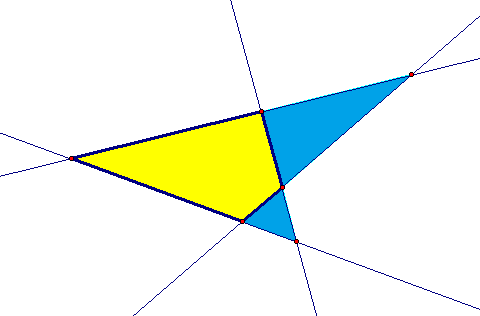
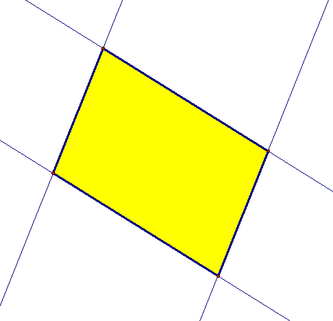
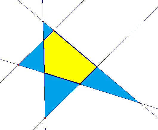
A few days ago, I came across the phrase, while surfing the Internet, “the extended quadrilateral has six vertices.” Not understanding this, I researched the matter, and found out what this phrase means. If the normal four vertices of a quadrilateral are placed such that the quadrilateral has no parallel sides, then two additional vertices are created when the four sides are extended as lines, as shown below. This gives a total of six vertices for this extended quadrilateral.

quad6

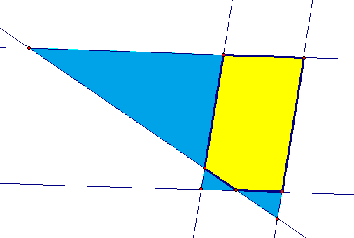
Of course, one need not position the vertices in this way. Trapezoids, by definition, have one pair of parallel sides. The non-parallel sides of an extended trapezoid still intersect outside this quadrilateral, creating a five-vertex situation.

quad5

The other option is the parallelogram, with two pairs of parallel sides. This eliminates additional vertices altogether, so there are only four.

quad4

This exhausts the possibilities, so the possible numbers of vertices for extended quadrilaterals are 4, 5, and 6.

Realizing this, of course, just raises other questions: what about other extended convex polygons? What are the numbers of possible intersections for such polygons with varying numbers of sides? Is there a pattern? To investigate this, I needed data, and started by taking a step back from quadrilaterals, to briefly consider extended triangles.

triangle

Extending the sides of any triangle creates no additional vertices, beyond the three which exist before the extension. This is a result of the fact that three is the maximum number of intersections created by three coplanar lines. Three is, therefore, for triangles, the only answer.

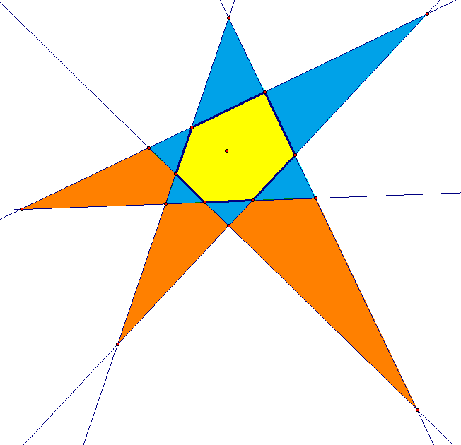
The next step: consider extended convex pentagons. I decided to start by maximizing the number of vertices, by having no parallel sides at all.

pent10

As you can see above, this produces ten vertices — five for the non-entended pentagon, plus five more formed by the entensions. To reduce this number, I simply moved vertices of the original, non-extended pentagon to eliminate external vertices, one at a time, by creating pairs of parallel sides.

pent9

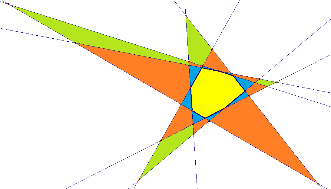
With one pair of parallel sides, as shown above, the number of vertices is reduced by one, from ten to nine.

pent8

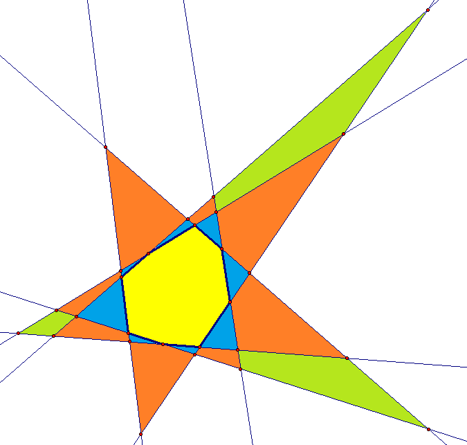
For pentagons, the maximum number of pairs of parallel sides is two, as shown above, which lowers the total number of vertices to eight. For pentagons, then, there are three solutions to this puzzle: 8, 9, and 10.

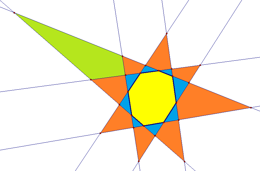
Next, I considered hexagons.

hex15

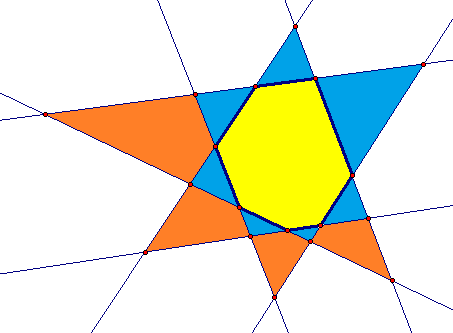
The extended hexagon above has no parallel sides, which gives it the maximum number of vertices:  fifteen. In the figure below, by contrast, there is one pair of parallel sides, reducing this number to fourteen.

hex14

hex13

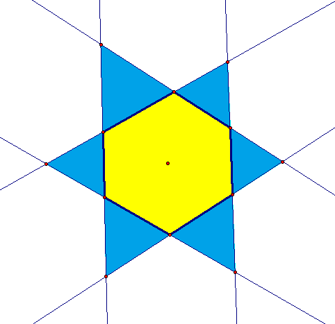
With two pairs of parallel sides, as shown above, this number again decreases by one, to thirteen. Three pairs of parallel sides is the maximum for hexagons, and is shown below; for this extended hexagon, there are twelve vertices.

hex12

For hexagons, then, there are four solutions:  15, 14, 13, and 12.

Still needing more data, I next investigated extended convex heptagons. With no parallel sides at all, as shown below, the total number of vertices is twenty-one.

hept21

hept20

If only one pair of parallel sides exist, there is one less vertex than the previous answer gave, and this number is twenty, as shown above. It is also possible for there to be two pairs of parallel sides, as shown below, and this yields nineteen vertices.

hept19

For heptagons, there is only one other option: three pairs of parallel sides. (A fourth pair would require eight sides.) This situation is shown below, and in it, there are eighteen vertices.

hept18

For heptagons, then, the solutions are four in number:  18, 19, 20, and 21.

Next: octagons. With no sides parallel, to obtain the maximum number of vertices (as shown below), there are twenty-eight of them.

oct28

In the diagram below, the solution immediately above is reduced by one, to twenty-seven, by making one pair of sides parallel.

oct27

The next solution is shown below, and is twenty-six. This is accomplished by making two pair of sides parallel.

oct26

To obtain twenty-five vertices, three pairs of sides are made to be parallel, as shown below.

oct25

Finally, twenty-four vertices, the minimum for octagons, requires all four pairs of opposite sides to be parallel. This solution is shown below.

oct24

Octagons, then, have five solutions:  24 to 28, inclusive.

Here is the data gathered above, in the form of a table, along with additional data obtained by extrapolation, work shown toward a generalized solution, and then that generalized solution itself, in three parts: one for triangles, one where the number of sides is even, and one where n, the number of sides, is odd, with n > 3.

hept21

Polygons Related to the Golden Ratio, and Associated Figures in Geometry, Part 2: Quadrilaterals

The golden ratio, also known as φ, has a value of [1 + sqrt(5)]/2, or ~1.61803. It is associated with a great many figures in geometry, and also appears in numerous other contexts. The most well-known relationship between a geometric figure and the golden ratio is the golden rectangle, which has a length:width ratio equal to the golden ratio. An interesting property of the golden rectangle is that, if a square is removed from it, the remaining portion is simply a smaller golden rectangle — and this process can be continued without limit.

golden rectangle

While the golden ratio is related to many polyhedra, this relationship does not always involve golden rectangles, but sometimes it does. For example, it is possible to modify a rhombicosidodecahedron, by replacing that figure’s squares with golden rectangles (with the longest side adjacent to the triangles, not the pentagons), to obtain a “Zomeball” — the node which is at the heart of the Zometool ball-and-stick modeling system for polyhedra, and other phenomena. The entire Zome system is based on the golden ratio. Zome kits are available for purchase at http://www.zometool.com, and this image of a Zomeball was found at http://www.graphics.rwth-aachen.de/media/resource_images/zomeball.png.

zomeball

In some cases, the relationship between a golden rectangle, and a polyhedron, is more subtle. For example, consider three mutually-perpendicular golden rectangles, each with the same center:

3 GOLDEN RECTANGLES

While this is not, itself, a polyhedron, it is possible to create a polyhedron from it, by creating its convex hull. A convex hull is simply the smallest convex polyhedron which can contain a given figure in space. For the three golden rectangles above, the convex hull is the icosahedron, one of the Platonic solids:

ICOSAl

In addition to the golden rectangle, there are also other quadrilaterals related to the golden ratio. For example, a figure known as a golden rhombus is formed by simply connecting the midpoints of the sides of a golden rectangle. The resulting rhombus has diagonals which are in the golden ratio.

golden rhombus

One of the Archimedean solids, the icosidodecahedron, has a dual called the rhombic triacontahedron. The rhombic triacontahedron has thirty faces, and all of them are golden rhombi.

Rhombic Triaconta

There are also other polyhedra which have golden rhombi for faces. One of them, called the rhombic hexacontahedron (or “hexecontahedron,” in some sources), is actually the 26th stellation of the rhombic triacontahedron, itself. It has sixty faces, all of which are golden rhombi.

Rhombic Triaconta 26th stellation

Other quadrilaterals related to the golden ratio can be formed by reflecting the golden triangle and golden gmonon (described in the post right before this one) across each of their bases, to form two other types of rhombus.

rhombi for penrose tilings

In these two rhombi, the golden ratio shows up as the side-to-short-diagonal ratio (in the case of the 36-144-36-144 rhombus), and the long-diagonal-to-side ratio (in the case of the 72-108-72-108 rhombus). These two rhombi have a special property:  together, they can tile a plane in a pattern which never repeats itself, but, despite this, can be continued indefinitely. This “aperiodic tiling” was discovered by Roger Penrose, a physicist and mathematician. The image below, showing part of such an aperiodic tiling, was found at https://en.wikipedia.org/wiki/Penrose_tiling.

500px-Penrose_Tiling_(Rhombi).svg

There are also at least two other quadrilaterals related to the golden ratio, and they are also formed from the golden triangle and the golden gnomon. The procedure for making these figures, which could be called the “golden kite” and the “golden dart,” is similar to the one for making the rhombi for the Penrose tiling above, but has one difference: the two triangles are each reflected over a leg, rather than a base.

kite and dart for for penrose tilings

In the case of this kite and dart, it is the longer and shorter edges, in each case, which are in the golden ratio — just as is the case with the golden rectangle. Another discovery of Roger Penrose is that these two figures, also, can be used to form aperiodic tilings of the plane, as seen in this image from http://www.math.uni-bielefeld.de/~gaehler/tilings/kitedart.html.

kitedart

There is yet another quadrilateral which has strong connections to the golden ratio. I call it the golden trapezoid, and this shows how it can be made from a golden rectangle, and how it can be broken down into golden triangles and golden gnomons. However, I have not yet found an interesting polyhedron, not tiling pattern, based on golden trapezoids — but I have not finished my search, either.

golden trapezoid

[Image credits:  see above for the sources of the pictures of the two Penrose tilings, as well as the Zomeball, shown in this post. Other “flat,” nonmoving pictures I created myself, using Geometer’s Sketchpad and MS-Paint. The rotating images, however, were created using a program called Stella 4d, which is available at http://www.software3d.com/Stella.php.]

Polygons Related to the Golden Ratio, and Associated Figures in Geometry, Part 1: Triangles

golden triangles

There are two isosceles triangles which are related to the golden ratio, [1 + sqrt(5)]/2, and I used to refer to them as the “golden acute isosceles triangle” and the “golden obtuse isosceles triangle,” before I found out these triangles already have other names –the ones shown above. The golden triangle, especially, shows up in some well-known polyhedra, such as both the great and small stellated dodecahedron. The triangles which form the “points” or “arms” of regular star pentagons (also known as pentagrams) are also golden triangles.

These triangles have sides which are in the golden ratio. For the golden triangle, it is the leg:base ratio which is golden, as shown above. For the golden gnomon, this ratio is reversed:  the base:leg ratio is φ, or ~1.61803 — the irrational number known as the golden ratio.

The angle ratios of each of these triangles are also unique. The golden triangle’s angles are in a 1:2:2 ratio, while the angles of the golden gnomon are in a ratio of 1:1:3.

Another interesting fact about these two triangles is that each one can be subdivided into one of each type of triangle. The golden triangle can be split into a golden gnomon, and a smaller golden triangle, while the golden gnomon can be split into a golden triangle, and a smaller golden gnomon, as seen below.

golden triangles 2

This process can be repeated indefinitely, in each case, creating ever-smaller triangles of each type.

Polyhedra which use these triangles, as either faces or “facelets” (the visible parts of partially-hidden faces) are not uncommon, as previously mentioned. The three most well-known examples are three of the four Kepler-Poinsot solids. In the first two shown below, the small stellated dodecahedron and the great stellated dodecahedron, the actual faces are regular star pentagons which interpenetrate, but the facelets are golden triangles.

Small Stellated Dodeca

Great Stellated Dodeca

The next example is also a Kepler-Poinsot solid: the great dodecahedron. Its actual faces are simply regular pentagons, not star pentagons, but, again, they interpenetrate, hiding much of each face from view. The visible parts, or “facelets,” are golden gnomons.

Great Dodeca

For another example of a polyhedron made of golden gnomons, I made one myself — meaning that if anyone else has ever seen this polyhedron before, this fact is unknown to me, although I cannot rule it out. I have not given it a name. It has thirty-six faces, all of which are golden gnomons. There are twelve of the larger ones, shown in yellow, and twenty-four of the smaller ones, shown in red. This polyhedron has pyritohedral symmetry (the same type of symmetry seen in the seam-pattern of a typical volleyball), and its convex hull is the icosahedron.

36 golden gnomons

[Picture credits: to create the images in this post, I used both Geometer’s Sketchpad and MS-Paint for the two still, flat pictures found at the top. To make images of the four rotating polyhedra, I used a different program, Stella 4d: Polyhedron Navigator. Stella is available for purchase, with a free trial download available, at http://www.software3d.com/Stella.php.]

A Polyhedron Featuring Twelve Regular Pentadecagons, and Twenty Regular Enneagons

152 faces featuring regular enneagons and pentadecagons

In the last post here, there were two polyhedra shown, and the second one included faces with nine sides (enneagons, also known as nonagons), as well as fifteen sides (pentadecagons), but those faces were not regular.

The program I use to manipulate polyhedra, Stella 4d (available at http://www.software3d.com/Stella.php),  has a “try to make faces regular” function included. When I applied it to that last polyhedron, in the post before this one, Stella was able to make the twenty enneagons and twelve pentadecagons regular. The quadrilaterals are still irregular, but only because squares simply won’t work to close the gaps of a polyhedron containing twenty regular enneagons and twelve regular pentadecagons. These quadrilaterals are grouped into thirty panels of four each, so there are (4)(30) = 120 of them. Added to the twelve pentadecagons and twenty enneagons, this gives a total of 152 faces for this polyhedron.

A Radial Tessellation of Regular Pentagons and Their Expanding Gap-Polygons

pentagonsI call this sort of thing a “radial tessellation” — it follows definite rules that resemble those for regular or semi-regular tessellations, but possesses, primarily, radial symmetry. It also has lines of reflective symmetry, but these lines all meet at the radial-symmetry central point, which, in this case, is inside the central pentagon.

Moving out from the central point, the first gap-polygons encountered are black rhombi. The gaps exist because the 360 degrees necessary to surround a point cannot be divided by a whole number of 108 degree angles, from the regular pentagons, without leaving a remainder. This remainder, from arithmetic, is manifested geometrically as a gap between pentagons.

After the rhombi, moving further from the center, appear purple, non-convex equilateral hexadecagons, then, after that, larger, red polygons with more sides and indentations, and then the next, even-more-complex polygons after that, in yellow. Off the edges of the screen, this increase in gap-polygon size and complexity continues without limit, provided the pattern shown is followed. Here is the “recipe” for producing it:

1. Begin with a regular pentagon. Locate its center, and use it as the center point for all rotations.

2. Designate the line containing an outer edge of your figure as a line of reflection.

3. Reflect your entire figure over the designation line of reflection.

4. Take the newly-reflected figure, and rotate it around the central point by 72 degrees. Next, perform this same rotation, using the newest figure produced each time, three more times.

5. Return to step 2.

A Tessellation Using Regular Pentagons and Hexagons, As Well As Two Types of Concave Polygon

tiling

Without even checking, I know that my automatic tweet about this post (as @RobertLovesPi) will be retweeted by the @HexagonBot on Twitter. Why? Because @HexagonBot retweets any tweet containing the word “hexagon,” or “hexagons.” I have absolutely no idea why other polygons lack their own Twitterbots, though.

A Euclidean Construction of a Regular Pentagon with a Given Edge Length

The most well-known method for constructing a regular pentagon causes it to be inscribed in a given circle with a known center. It’s easy to find, on-line or in textbooks, and I will not be reproducing that construction here.

Because the diagonals and sides of a regular pentagon are in the golden ratio, it is also not difficult to construct a golden rectangle, and then use it to construct a regular pentagon. Given the ease of finding instructions for constructing a golden rectangle elsewhere, though, I’m not posting that construction here, either. This one begins with two distinct points, A and B, and the segment which connects them. The goal here is to start with only that, and then construct a regular pentagon, with sides of length AB, using only the methods permitted for Euclidean constructions.

pent1

After segment AB has been drawn, the next step is to continue it, in both directions, to form line AB. Next, construct two circles, each with radius AB: one centered on A, and the other centered on B. These circles must intersect at two points, labeled C and D, as shown above. The next step is to construct line CD, and label, as point E, the intersection of lines AB and CD. This is the well-known procedure for constructing the perpendicular bisector of a segment, so E is the midpoint of segment AB, and the four angles with vertices at E are each right angles.

pent2

Next, construct a circle, centered on E, with radius AE. Label, as point F, the intersection of this circle with segment CE. After than, construct a circle, centered on B, with radius BE. This circle intersects line AB at two points, one of which is already labeled E. Label, as point G, the other such intersection. At this time, because they are all radii of equal-sized circles, the following lengths are equal:  AE, BE, BG, and EF. Segment EG, however, is twice as long as any of these shorter and equal-length segments, since it is a straight segment formed by combining non-overlapping segments BE and BG. Since the same can be said for segment AB as well — its length equals AE + BE, or 2AE by substitution and addition — it follows that AB = EG. The next step is to construct line FG, which necessarily includes segment FG. Since segment FG is the hypotenuse of right triangle EFG, which has one leg (segment EG) which is twice as long as the other leg (segment EF), it follows, from the Pythagorean Theorem, that the distance FG is equal to the distance EF times the square root of five. Next, construct a circle which is centered at F, and has segment EF for a radius. Label the intersections of line FG, and this circle, as points H and K, as shown above, with K being the closer of the two to point G. Now there are two new segments, FH and FK, which, because they are radii of the same circle as segment EF, are each equal in length to segment EF, as well as to segments AE, BE,  and GB, each of which were already shown to be equal in length to EF, and half as long as either of the equal-length segments EG and AB.

pent3

The next step is to construct a circle, centered at G, with radius EG. After that, consider the collinear and adjacent segments FH and FG, which, together, compose segment GH. FH is one of the several segments known to be half as long as AB, and FG’s length is already known to be equal to this shorter length (that of segments EF, FH, AE, etc.) times the square root of five. By the segment addition postulate, then, segment GH’s length is equal to the length of one of the shorter segments AE, EF, etc., times the sum of one and the square root of five. This length, GH, will be used as the diagonal-length of the regular pentagon, because GH’s length, and the edge length originally provided (AB), are in the golden ratio, since segment AB is twice as long as segment EF, and GH is equal to EF times the sum of one and the square root of five. GH is the radius of the next circle to construct, and that circle should be centered at H. This circle, the largest yet constructed, intersects the radius-EG circle centered at G at two points. One of these intersection-points, on the same side of line AB as right triangle EFG, need not be labeled, but the other one, on the other side of line AB, should be labeled as point J, as shown above. Segments GJ and EG, then, have equal lengths, for they are radii of the same circle — and the distance EG has already been shown to be equal to the distance AB, so GJ = AB as well. The segments GJ and AB are highlighted in pink in the diagram above, with their lengths shown, in order to provide additional evidence that their lengths are equal.

pent4

In the diagram above, segment GJ is shown in bold, because it is a side of the pentagon being constructed. Segment HJ is then constructed, and is also shown in bold, for it is a diagonal of that same pentagon, having the correct length by virtue of being a radius of the same circle as segment GH, which was already shown to have the correct length for a diagonal of the pentagon. The next step is to locate point L, which will be a vertex of the pentagon. To do that, construct a circle of radius HK, centered on H. Because segment HK is formed by the non-overlapping, adjacent, and collinear segments FH and FK, each of which has the same length as AE or AB, it follows that HK, the radius of the last circle constructed, is equal in length to both AB and GJ, with this distance being the side-length of the pentagon being constructed.

Next, construct a circle which has radius GH (the diagonal-length of the pentagon), and is centered at G. This circle, and the already-constructed circle with radius HK which is centered at H, intersect at two points. Label one of these points of intersection (the one on the same side of line AB as point J) as point L, as shown above, and then construct pentagon-sides HL and JL, also shown in bold in the figure above. (Also shown: measured lengths of all segments rendered in bold thus far, as well as AB.) Of these last two circle-intersection points, one has now been labeled as point L. The next step is to label the other such intersection as point M, as shown in the diagram below.

pent5

Once point M is located, the remaining sides and diagonals of regular pentagon GJLHM can be constructed, as shown above, in bold, simply by connecting each remaining unconnected pair of pentagon-vertices with a segment. The lengths of all bold segments, plus the original segment AB, are also shown above. As you can see, all five sides have length equal to the length of segment AB, while all five diagonals have a length greater than that of AB, but one which is constant throughout the set of diagonals.

pent6

In the diagram above, no new objects have been constructed using the Euclidean tools, but the pentagon has been given color, and a check of the diagonal-length to side-length ratio has been performed. As you can see, in the uppermost calculation, the decimal approximation for this distance-ratio is given as 1.61803. The same result is obtained, in the second calculation shown, when the sum of one, and the square root of five, is divided by two — and, since this is the definition of the golden ratio, obtaining the same result, for both of these calculations, provides supporting evidence for the validity of this construction.

pent7

To perform one more test of this construction — one only possible with a virtual compass and straightedge, such as Geometer’s Sketchpad, the one I used here — points A and/or B can be moved around. I chose to move them both, and I also increased the distance between them. As you can see, this increased all the side and diagonal lengths, as well as the length of the original segment, AB. However, segment AB still has the same length as all five pentagon sides. Also, all five diagonals, while they do have a longer length than any side, still have lengths equal to each other. Also, the diagonal-length to side-length ratio remains constant, at the value of the golden ratio, even though the actual distances all changed when A and B were moved. The construction, and its explanation, are now complete.