On Binary Planets, and Binary Polyhedra

Faceted Augmented Icosa

This image of binary polyhedra of unequal size was, obviously, inspired by the double dwarf planet at the center of the Pluto / Charon system. The outer satellites also orbit Pluto and Charon’s common center of mass, or barycenter, which lies above Pluto’s surface. In the similar case of the Earth / Moon system, the barycenter stays within the interior of the larger body, the Earth.

I know of one other quasi-binary system in this solar system which involves a barycenter outside the larger body, but it isn’t one many would expect: it’s the Sun / Jupiter system. Both orbit their barycenter (or that of the whole solar system, more properly, but they are pretty much in the same place), Jupiter doing so at an average orbital radius of 5.2 AU — and the Sun doing so, staying opposite Jupiter, with an orbital radius which is slightly larger than the visible Sun itself. The Sun, therefore, orbits a point outside itself which is the gravitational center of the entire solar system.

Why don’t we notice this “wobble” in the Sun’s motion? Well, orbiting binary objects orbit their barycenters with equal orbital periods, as seen in the image above, where the orbital period of both the large, tightly-orbiting rhombicosidodecahedron, and the small, large-orbit icosahedron, is precisely eight seconds. In the case of the Sun / Jupiter system, the sun completes one complete Jupiter-induced wobble, in a tight ellipse, with their barycenter at one focus, but with an orbital period of one jovian year, which is just under twelve Earth years. If the Jovian-induced solar wobble were faster, it would be much more noticeable.

[Image credit: the picture of the orbiting polyhedra above was made with software called Stella 4d, available at this website.]

Thirty-Four Rotating, Convex, and Non-Chiral Polyhedra with Icosidodecahedral Symmetry

Most in the field call this type of symmetry “icosahedral,” but I prefer the term George Hart uses — along with “cuboctahedral” in place of “octahedral.”

Each polyhedral image here was created with Stella 4d: Polyhedron Navigator. At this linked page, you can try a trial version of that program for free.

12 icosagons and stuff

Dual of Convex huull

272 faces in 12 reg dec & 120 scalene triangles and 60 isos triangles and 60 isos traps and 20 reg hexagons

Convex hnbghjull

Convex hull 20 8 and 12

By the way, when I described these polyhedra, in this post’s title, as non-chiral, I was not referring to the coloring-schemes used here, many of which obviously are chiral, but only the shapes themselves.

Convex hull LP

convex hull of synthetic comet nucleus

Dual of Convex hull

Convexxx hull

Convhgfehgx hull

That 10 GB space-upgrade, which most bloggers don’t ever need, is really coming in handy right now. In other words, some of these .gif files are huge!

Convhgfex hull

Dual of Chgonvex hulgfl

Dual of Chgonvex hull

Dual of Cjhfjonvex hull

Dualhhc of Convex hull

Why, yes, I am including some words after every fifth polyhedron. That will help, later, when I count them for the title of this post.

Dual of Conjhvex hull

enneagons and kites

Enneagons, Pentagon, isostraps, and rectangles

exansiaon Convex hull

Expanded GRID

I’m not sure why that last one is spinning the opposite direction from the others. Perhaps this polyhedron is trying to start a trend. On the other hand, it could just simply upside-down.

Faceted Stellated Dual of Convex hull

metaexpanded RID

ID variation

intermediate form

jdshfgs

That’s twenty-five so far.

metaRID

pentadecagons two types hexagons and trapezoids

RID variant

RTC and RID blend

Stellated Poly

Clearly, I should have checked the number of files in that file folder before deciding to simply post them all together, based on what they have in common. That’s thirty so far.

sixty pentagons and twenty hexagons

twenty regular dodecagons

Unnabsghfmed

what is this thing

Order-Six Radial Tessellations of the Plane, Using Elongated and Equilateral Hexagons, Rendered with Twelve Different Coloring-Schemes

I explored radial tessellations of the plane, using only hexagons, in this earlier post. Order-three tessellations of this type are the familiar regular-hexagon tessellations of the plane. With higher-order all-hexagon radial tessellations, though, the hexagons must be elongated, although they can still remain equilateral, and all congruent, with bilateral symmetry. In that previous post, examples were shown of order 4, 5, and 8, in addition to the familiar order-3 regular-hexagon tessellation.

This left out order-6, of which I show many examples below. As it turns out, this particular radial tessellation lends itself particularly well to a variety of coloring-schemes. In the first picture, the construction-circles, -points, and -lines I used are shown; in the rest, they are hidden.

No upper limit exists to the order-number of these all-hexagon radial tessellations — although the larger that number gets, the thinner the hexagons become, relative to their edge length. At some point (which I expect would vary from person to person), as the order-number increases, the hexagons needed will become so thin that they will no longer be recognizable as hexagons.

frequency 6 radial tessellation of hexagons with construction lines

Next, with construction artifacts hidden, are some two-color designs I found.

frequency 6 radial tessellation of hexagons without construction lines 2-color

frequency 6 radial tessellation of hexagons without construction lines 2-color version two

Here are some which use three colors each:

frequency 6 radial tessellation of hexagons without construction lines 3-color version colored by another system

frequency 6 radial tessellation of hexagons without construction lines 3-color version two

frequency 6 radial tessellation of hexagons without construction lines 3-color

frequency 6 radial tessellation of hexagons without construction lines 3-color version colored by rings

I also found some four-color patterns with interesting symmetry:

frequency 6 radial tessellation of hexagons without construction lines

frequency 6 radial tessellation of hexagons without construction lines. four colors version 2png

Finally, here are some which each use six colors.

frequency 6 radial tessellation of hexagons without construction lines 6-color version two

frequency 6 radial tessellation of hexagons without construction lines 6-color version colored by another system

frequency 6 radial tessellation of hexagons without construction lines 6-color

Two Different Versions of an Expanded Snub Dodecahedron, Both of Which Feature Regular Decagons

The snub dodecahedron, one of the Archimedean solids, can be expanded in multiple ways, two of which are shown below. In each of these expanded versions, regular decagons replace each of the twelve regular pentagons of a snub dodecahedron.

exp sn dodeca 2

Exp Sn Dodaca

Like the snub dodecahedron itself, both of these polyhedra are chiral, and any chiral polyhedron can be used to create a compound of itself and its own mirror-image, Below, you’ll find these enantiomorphic-pair compounds, each made from one of the two polyhedra above, together with its own reflection.

exp sn dodeca 2 compound of enantiomophic pair

exp sn dodaca Compound of enantiomorphic pair exp snub dodeca

All four of these images were created using Stella 4d: Polyhedron Navigator, software available (including a free trial download) at this website.

On Pertrigonometric Functions

Pertrigonometric functions are modifications of the three primary trigonometric functions. Unlike the familiar sine, cosine, and tangent functions, the “pertrig” functions include triangle perimeter in their right-triangle-based definitions, which are given in the bulleted list below. The longer form of “pertrigonometric functions” is “perimeter-based trigonometric functions,” and the shorter, informal version is “pertrig functions.”

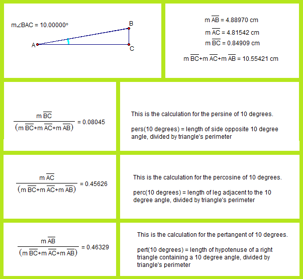
  • The persine of an acute angle (abbreviated “pers”) equals the length of the side opposite that angle, in a right triangle, divided by the triangle’s perimeter.
  • The percosine of an acute angle (abbreviated “perc”) equals the length of the leg adjacent to that angle, in a right triangle, divided by the triangle’s perimeter.
  • The pertangent of an acute angle (abbreviated “pert”) equals the length of the hypotenuse of a right triangle containing this acute angle, divided by the triangle’s perimeter.

After defining these terms, I used Geometer’s Sketchpad to construct a right triangle containing a 10º angle, and then used the “measure” and “calculate” functions to find the values of pers(10º), perc(10º), and pert(10º). Since these are ratios, they would have the same values shown for larger or smaller right triangles which contain 10º angles.

pertrig functions

An observation: the pertangents of complementary angles are equal. Why? Because complementary angles appear in all right triangles, as pairs of acute angles in the same triangle. For each such complementary angle pair, therefore, the same triangle is used to define pertangent. The hypotenuse/perimeter ratio (which is pertangent) would, it follows, remain unchanged — because both its numerator and denominator remain unchanged.  This relationship does not hold for the tangent function; instead, the tangents of complementary acute angles are reciprocals of each other.

Of course, I wanted to know more than just the pers, perc, and pert values for 10º, but I had no desire to repeat the same calculations, many more times, to form a table. Instead, I simply graphed the functions, again using Geometer’s Sketchpad. The units on the x-axis are degrees, not radians.

pertrig functions B

In the graph above, the dark blue curve is the persine function, with the sine function in light blue, for comparison. Similarly, percosine is shown in red, with cosine shown in pink. Finally, pertangent is shown with a heavy, dark green curve, while tangent is shown as a thinner, light green curve.

Entering the equations for these curves was a little tricky, due to the fact that I wanted this graph to venture beyond 0 and 90 degrees, in both directions, on the x-axis. When that is done, the unit circle must be used (in place of right-triangle based definitions), simply because no right triangles contain angles outside this range. The radius of the unit circle is 1, by definition, and that is the hypotenuse of the right triangle which exists in the zero-to-ninety degree part of the domain of the graph above. As a consequence of setting the length of the hypotenuse of each right triangle at 1, the side opposite the angle in question (used for persine) becomes, simply, the sine of that angle, while the adjacent leg’s length is the angle’s cosine. It then follows that the perimeter (the denominator of the pers, perc, and pert ratios) is equal to sin(x) + cos(x) + 1.

Calculations are shown on the graph above, and you can click on the graph to enlarge it, to make them more readable. In these calculations, one more adjustment had to be made, and that was to the perimeter portion of each pertrigonometric ratio. Using sin(x) + cos(x) + 1 works fine for perimeter, for the zero-to-ninety degree portion of the domain, but, outside that, negative numbers intrude, for values of sin(x) and/or cos(x). It is my contention that triangle perimeter only makes sense as a sum of absolute values of a triangle’s three side lengths. To obtain absolute values for both sin(x) and cos(x) in the perimeter-part of each calculation, then, I simply squared each of these two functions, and then took the square roots of those squares. The result of this can be seen on the graph, in the curve for the pertangent function, which resembles a child’s drawing of waves in the ocean. On the y-axis, it never reaches as low as 0.4, and its maximum value is clearly exactly 0.5 — at the sharp “wave peaks.” At the (smooth) troughs, the actual minimum is equal to the square root of two, minus one, or ~0.414, although I have not yet figured out exactly why that is the case — I simply noticed it on the graph — but, to investigate it further, I know where to look: the 45-45-90 triangle, since these minima are hit when x = (45 ± 90n) degrees, where n is any integer. The pertangent function has the shortest period of all the functions shown above, at a mere 90º. For tangent, by contrast, the period is 180º. All four of the other functions shown have periods of a full 360º.

It is striking that the pertangent and tangent curves bear little resemblance to each other, while marked resemblances do exist between the persine and sine curves, as well as between the percosine and cosine curves. In informal terms, the persine curve is a shorter and spikier (but still recognizable) version of the sine curve (vertically, with the amplitude exactly one-half as great for the shorter persine curve, relative to the sine curve), but, horizontally, the two curves are synchronized. The same relationship holds for the percosine and cosine curves. Also, it is well-known that the cosine curve is simply the sine curve, phase-shifted one-quarter cycle (or 90º, or π/2 radians) to the left. This phase-shift relationship between the cosine and sine curves holds, precisely, for the percosine and persine curves.

There is a simple reason why persine, percosine, and pertangent all peak at exactly y = ½. All three functions generalize, for acute angles, to this ratio — (some side of a right triangle)/(perimeter of that same triangle) — and no side of any triangle can ever exceed, nor even reach, half that same triangle’s perimeter. In all three cases, the maximum y-value is only reached, even in the zero-to-ninety degree portion of the domain, for “degenerate cases” — angles of 0º or 90º, which are, of course, not acute angles at all. Interpreted as triangles, these are cases where either a triangle becomes so short that it collapses to a single segment, or the opposite degenerate situation: two parallel lines, connected by a single segment. If you try to make either (or both) of the acute angles in a right triangle into an additional right angle, after all, that’s what you get.

To my knowledge, no one has described these pertrigonometric functions before, by this or any other name, although I could be wrong. (If I am wrong on this point, please let me know in a comment.) Regardless of whether this is their first appearance, or not, I did not invent them. The reason for this is simple: nothing in mathematics is ever “invented” — only discovered — for mathematics existed long before human beings existed, let alone started writing things down. How do I know this? Simple: there was a universe here before there were people, and all evidence indicates that it operated under the same laws of physics we observe today — and all evidence to date also indicates that those laws are mathematical in nature. Therefore, with the “pertrig” functions, I either discovered them, or, if they have been found before, then I independently rediscovered them.

Finally, I’ll address that question so often asked, about numerous things, in mathematics classes: what are these pertrigonometric functions used for? As far as I know, the answer in this case, so far, is absolutely nothing, other than delighting me by their very existence. It is possible that this may change, for someone might find a way to make a profitable application of these functions — and I won’t get any money if they do, either, for I am not copyrighting any of this. Nothing in mathematics is subject to ownership.

Honestly, though, I hope no one ever finds any practical, “real-world” use, at all, for pers, perc, or pert. Right now, they are pure mathematical ideas, unsullied by tawdry, real-world applications, and, well, I like that. I am far from the only person who ever had such an attitude about a mathematical idea, either — such views are actually fairly common in the mathematical community. Most of those who try to discover previously-unseen things in mathematics do so solely, or primarily, for one reason: the joy of discovery, in its purest form.

Slowly Rotating Hyperdodecahedron

This is the hyperdodecahedron, or 120-cell, one of the six four-dimensional analogs of the Platonic solids. It’s been shown on this blog before, but this image has one major change: a much slower rotational speed. It is my hope that this will help people, including myself, with the difficult task of understanding four-dimensional objects.

5-Hi, 120-cell, Hecatonicosachoron

This image was created using Stella 4d, a program you can try, as a free trial download, at this website.

Trinary Rhombicosidodecahedra

Faceted Augmented Rhombicosidodeca

This image of three rhombicosidodecahedra “orbiting” a common center was made with Stella 4d, a program you may try for free at this website.

Tidally Locked Binary Icosidodecahedra

binary icosidodecahedra

I’ve been trying to figure out for over a year how to make images like the one above, without having holes in the two polyhedra, facing each other. At last, that puzzle of polyhedral manipulation using Stella 4d (software available at this website) has been solved: use augmentation followed by faceting, rather than augmentation followed by simply hiding faces.

Two Similar Polyhedra with Icosidodecahedral Symmetry

octagons and kites

Stellated Chjhonvex hull

Both of these were made using Stella 4d, software you can try at this website.

Three Different Depictions of the Compound of Five Cubes

The most common depiction of the compound of five cubes uses solid cubes, each of a different color:

Cubes 5

This isn’t the only way to display this compound, though. If the faces of the cubes are hidden, then the interior structure of the compound can be seen. An edges-only depiction, still keeping a separate color for each cube, looks like this:

Cubes 5 edges

If these thin edges are then thickened into cylinders, that makes a third way to depict this polyhedral compound. It creates a minor problem, though: edges-as-cylinders looks awful without vertices shown as well, and the best way I have found to depict vertices, in this situation, is with spheres. With vertices shown as spheres, however, a sixth color, only for the vertex-spheres, is needed. Why? Because each vertex is shared by six edges: three from a cube of one color, and three from a second cube, of a different color.

Cubes 5 thick edges

Finally, here are all three versions, side-by-side for comparison, and with the motion stopped.

cover

All images in this post were created using Stella 4d: Polyhedron Navigator, software you may try for free at this website.